L3DAS23 dataset details
The datasets of both tasks share a common basis: the techniques adopted for generating it.
We used Soundspaces 2.0 [1] to generate Room Impulse Responses (RIRs) and images in a selection of simulated 3D houses from the Habitat - Matterport 3D Research Dataset [2]. Each simulated environment has a different size and shape, and includes multiple objects and surfaces to which specific acoustic properties (i.e., absorption, scattering, transmission, damping) are applied.
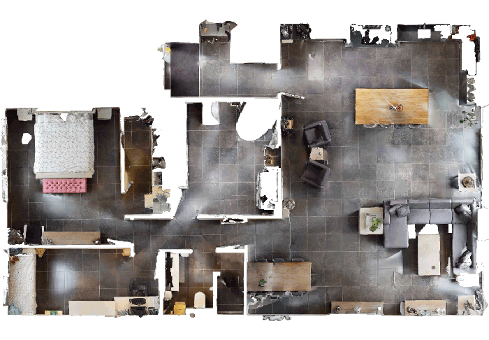
Figure 1: example of simulated environment from the Habitat - Matterport 3D Research Dataset. Image source: aihabitat.org
Recording procedure
We placed two Ambisonics microphones in 443 random positions of 68 houses and generated B-Format ACN/SN3D impulse responses of the rooms by placing the sound sources in random locations of a cylindrical grid defining all possible positions. The microphone and sound locations have been selected according to specific creteria, such as a minimum distance from walls and objects and a minimum distance between mic positions in the same environment.
One microphone (mic A) lies in the exact selected position, and the other (mic B) is 20 cm distant towards the x dimension of the RF of mic A. Both are shown as blue and orange dots in the topdown map in Fig. 2. Both microphones are positioned at the same height of 1.6 m, which can be considered as the average ear height of a standing person. The capsules of both mics have the same orientation.
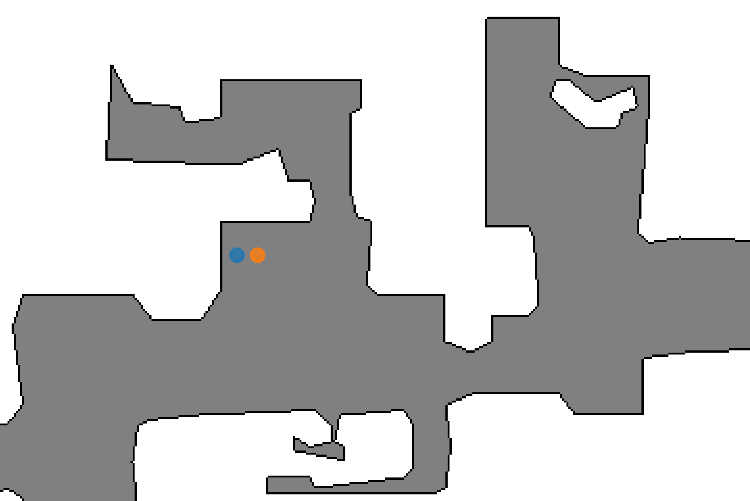
Figure 2: topdown map showing mic A (blue dot) and mic B (orange dot). Microphones can only be placed on the gray area (i.e., the area where no obstacles are located, namely the navigable area). On the contrary, sounds can be placed also outside the gray area, as long as they do not collide with objects and remain within the perimeter of the environments.
In every room, the speaker placement is performed according to five concentric cylinders centred in mic A, where the single positions are defined following a grid that guarantees a minimum euclidean distance of 50 cm between two sound sources placed at the same height.
The radius of the cylinders ranges from 1 m to 3 m with a 50 cm step and all have 6 position layers in the height dimension at 0.4 m, 0.8 m, 1.2 m, 1.6 m, 2 m, 2.4 m from the floor, as shown in Figure 3.
A sound can therefore be re produced in a room in any of the 700+ available positions (300k+ total positions in the selected environments), to which should be subtracted all those positions that collide with objects or exceed the room space. Figure 4 shows an example of source positioning at 0.4 m above the floor: the green dots represents accepted position (in this case, all positions within the room that do not collide with the sofa and the two armchairs), while the red dots show discarded positions.
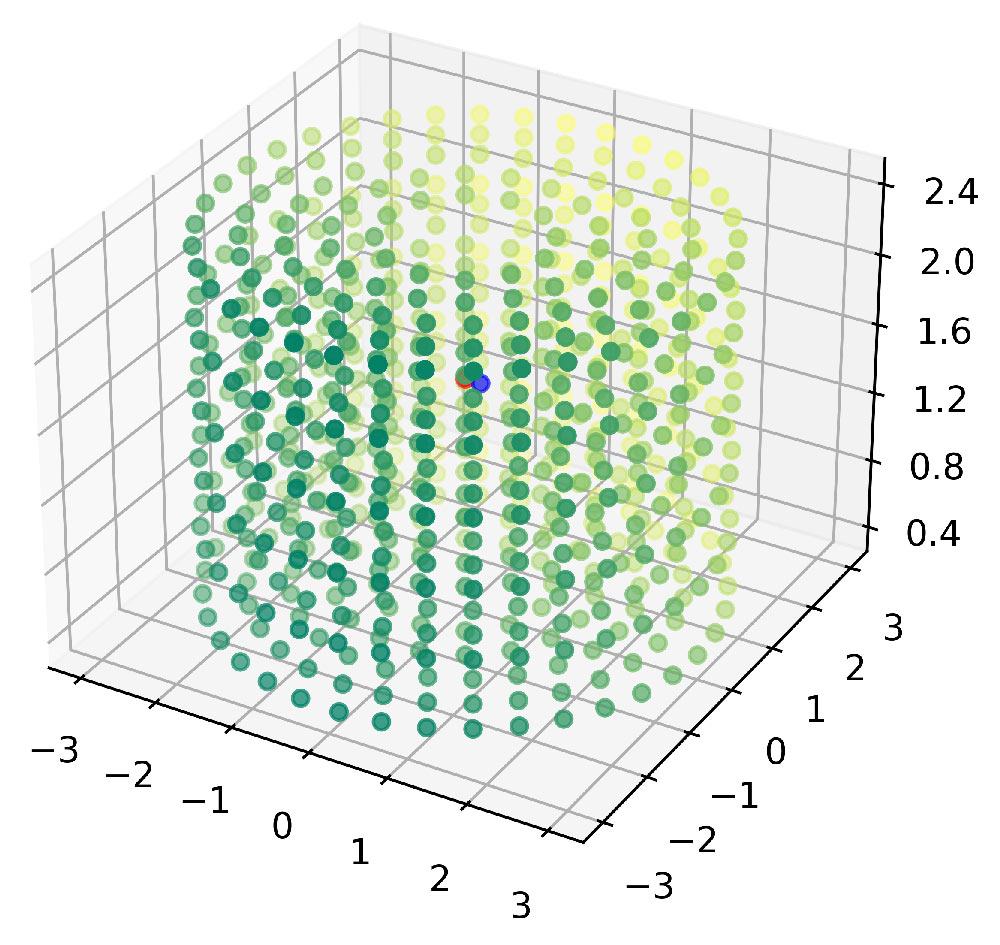
Figure 3: all the concentric cylinders. The partially visible red and blu dots represent mic A and B.
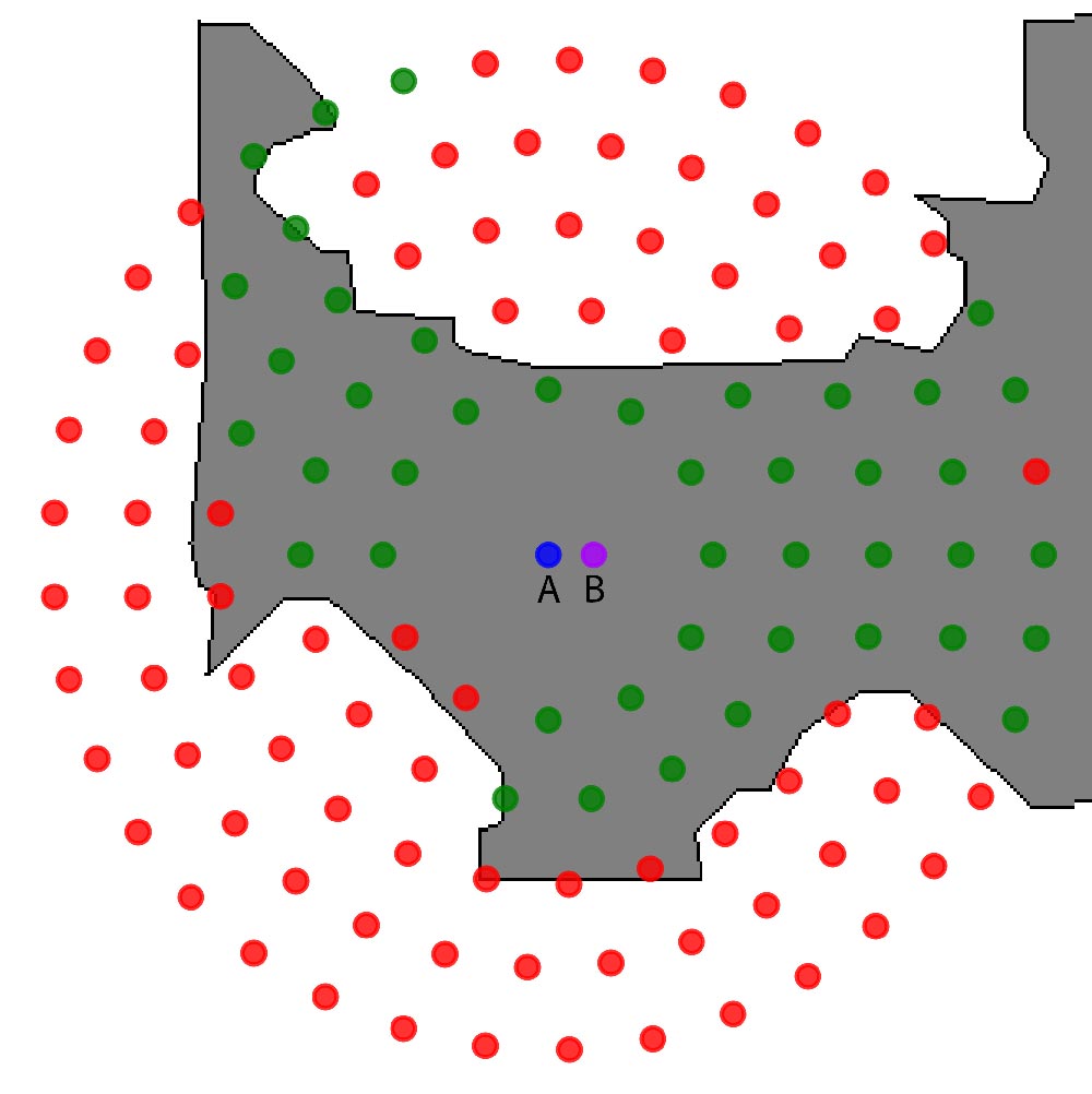
Figure 4: accepted source positions in green, discarded positions in red for one height level.
No constraint is placed on the need to have the sound source in the microphone's view (and thus a direct sound). A sound could then be placed behind an obstacle (such as a column in the center of a room).
Each speaker position is identified in cylindrical coordinates w.r.t. microphone A by a tuple (ρ, θ, z), where ρ is in the range [1.0, 3.0] (with a 0.5 step) and z in [-1.2, +0.8] (with a 0.4 step). θ is in the range [0°, 360°), with a step that depends on the value of ρ and is chosen so to satisfy the minimum euclidean distance between sound sources (θ = 0° for frontal sounds). All labels are consistent with this notation; elevation and azimuth or euclidean coordinates are however easily obtainable.
To make things more straightforward, we specify below in visual and written form how the coordinates used are defined and how to switch from one notation to another.
Figure 5 visually represents the tuple (ρ, θ, z). The orange dot in the picture is mic A and the black dot is a speaker placed on one of the concentric cylinders. ρ represents the distance of a sound source from mic A, θ is the angle from the Y axis, z is the height relative to mic A.
As shown in Figure 6, mic B is on the X-axis and thus in position (0.2, 0, 0) of a local coordinate system. Being frontal to the hearer, sounds placed on the Y-axis have θ = 0 in the dataset. θ is therefore calculated with respect to the Y-axis to comply with this principle. This has a direct impact on the way in which it is possible to switch from one notation to another. In the case of switching from cylindrical to euclidean coordinates, for example, the following formulas will be needed:
x = - ρ · sin(θ)
y = ρ · cos(θ)
z = z
Models can be trained using labels converted to the teams' preferred notation. In such cases, however, for the purposes of participation in the Challenge, the results must be conformed to our primary notation (cylindrical coordinates expressed as above) before being submitted.
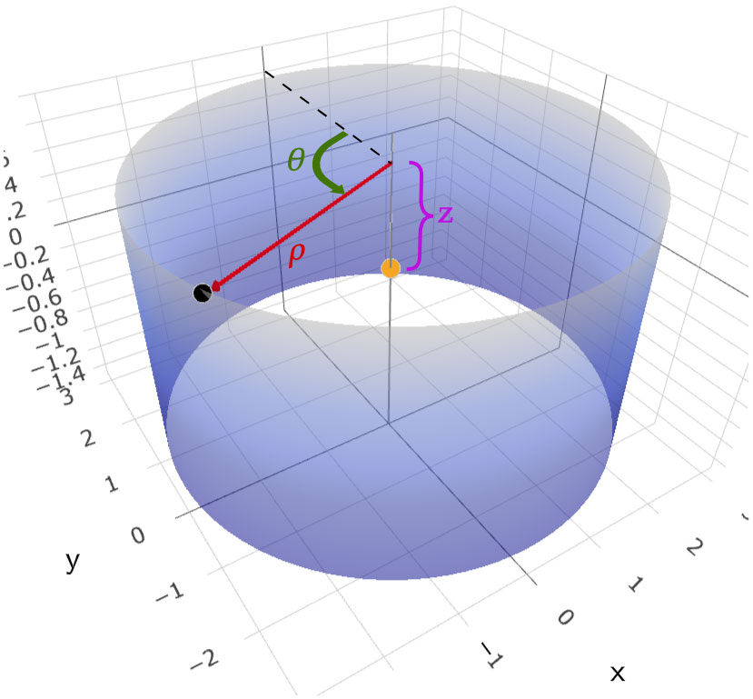
Figure 5: (ρ, θ, z) for one speaker position (black dot). Mic A is represented as an orange dot.
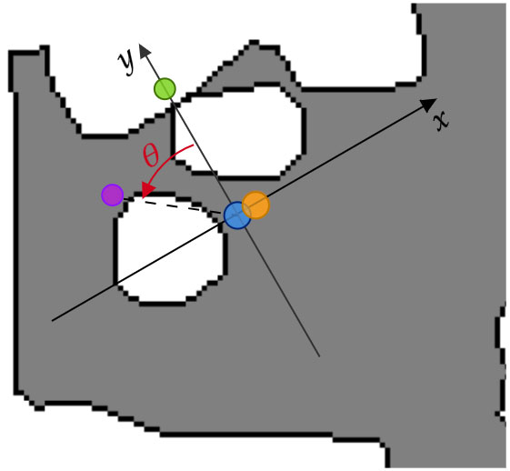
Figure 6: mic A (blue dot) is positioned at the center of the axes, mic B is at position (0.2, 0, 0), a frontal sound source standing on the Y-axis (green dot) has θ = 0, while a non-frontal sound source (like the on in purple) has a non-zero θ measured from the Y-axis.
The dataset is divided in two main sections, respectively dedicated to the challenge tasks. We provide normalized raw waveforms of all Ambisonics channels (8 signals in total) as predictors data for both sections, the target data varies significantly. Moreover, we created different types of acoustic scenarios, optimized for each specific task.
We split both dataset sections into: a training set (80 hours for SE and 5 hours for SELD) and a test set (7 hours for SE and 2.5 hours for SELD), paying attention to create similar distributions. The train set of the SE section is divided in two partitions: train360 and train100, and contain speech samples extracted from the correspondent partitions of Librispeech (only the sample up to 12 seconds). All sets of the SELD section are divided in: OV1, OV2, OV3. These partitions refer to the maximum amount of possible overlapping sounds, which are 1, 2 or 3, respectively.
Audio-visual tracks
In addition to the Ambisonics recordings, the dataset provides, for each microphone position in the rooms, an image of size 512x512 px, representing the environment in front of the main microphone (mic A). We derived these images by virtually placing a RGB sensor at the same height and orientation as microphone A, and with a 90-degree field of view. An example is shown below in Figure 7.
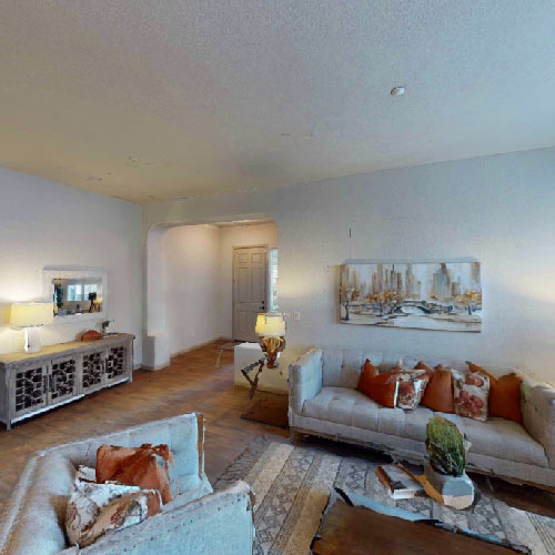
Figure 7: Example of a simulated view of the environment in front of the microphone
Since the microphone is placed in multiple different environments, the models will have to perform the tasks by adapting to different reverberation conditions. We expect higher accuracy/reconstruction quality in the case of the audio-visual track, especially when taking advantage of the dual spatial perspective of the two microphones.
The images are obtained in simulated environments, so they may have inaccuracies on the characterization of some elements, such as furniture. Figure 5, for example, features a floating book and vase. In addition, portions of open space are represented with black pixels.
This track should be regarded as highly experimental and as a way to investigate the integration of images in the more classical context of 3D SE and 3D SELD. We are already working to improve the visual part in future versions of the L3DAS dataset.
[1] Changan Chen, Carl Schissler, Sanchit Garg, Philip Kobernik, Alexander Clegg, Paul Calamia, Dhruv Batra, Philip W Robinson, and Kristen Grauman, “Soundspaces 2.0: A simulation platform for visual-acoustic learning,” in NeurIPS 2022 Datasets and Benchmarks Track, 2022.
[2] Santhosh Kumar Ramakrishnan, Aaron Gokaslan, Erik Wijmans, Oleksandr Maksymets, Alexander Clegg, John M Turner, Eric Undersander, Wojciech Galuba, Andrew Westbury, Angel X Chang, Manolis Savva, Yili Zhao, and Dhruv Batra, “Habitat-matterport 3D dataset (HM3d): 1000 large-scale 3D environments for embodied AI,” in Thirty-fifth Conference on Neural Information Processing Systems Datasets and Benchmarks Track, 2021